Customize BERTopic

Introduction

This notebook shows how to customize the different parts of the BERTopic pipeline: Embeddings, UMAP and HDBSCAN. See this Explainer and tutorial by pinecone.io) for details.

Imports and Login

import pandas as pd
import numpy as np
from tqdm.auto import tqdm
import json
from bertopic import BERTopic
from sentence_transformers import SentenceTransformer
import matplotlib.pyplot as plt
import seaborn as sns
import time
import torch
import umap
import hdbscan

Load publication data

df = pd.read_csv(INPUT_FILE)

df = df.drop_duplicates(subset=["doi"])\
            .dropna(subset=["doi", "abstract"]).reset_index(drop=True)
sentences = (df["title"] + " " + df["abstract"]).values

Embeddings

Compute or load sentence embeddings

if COMPUTE_EMBEDDINGS:
  embedding_model = SentenceTransformer('allenai-specter')
  embeddings = embedding_model.encode(sentences, normalize_embeddings=True)
  np.save(OUTPUT_FILE_TOPICS_EMBEDDINGS, embeddings)
else:
  embeddings = np.load(OUTPUT_FILE_TOPICS_EMBEDDINGS)

Sample embeddings

perm = torch.randperm(embeddings.shape[0])
idx = perm[:3000]
samples = embeddings[idx, :]

UMAP

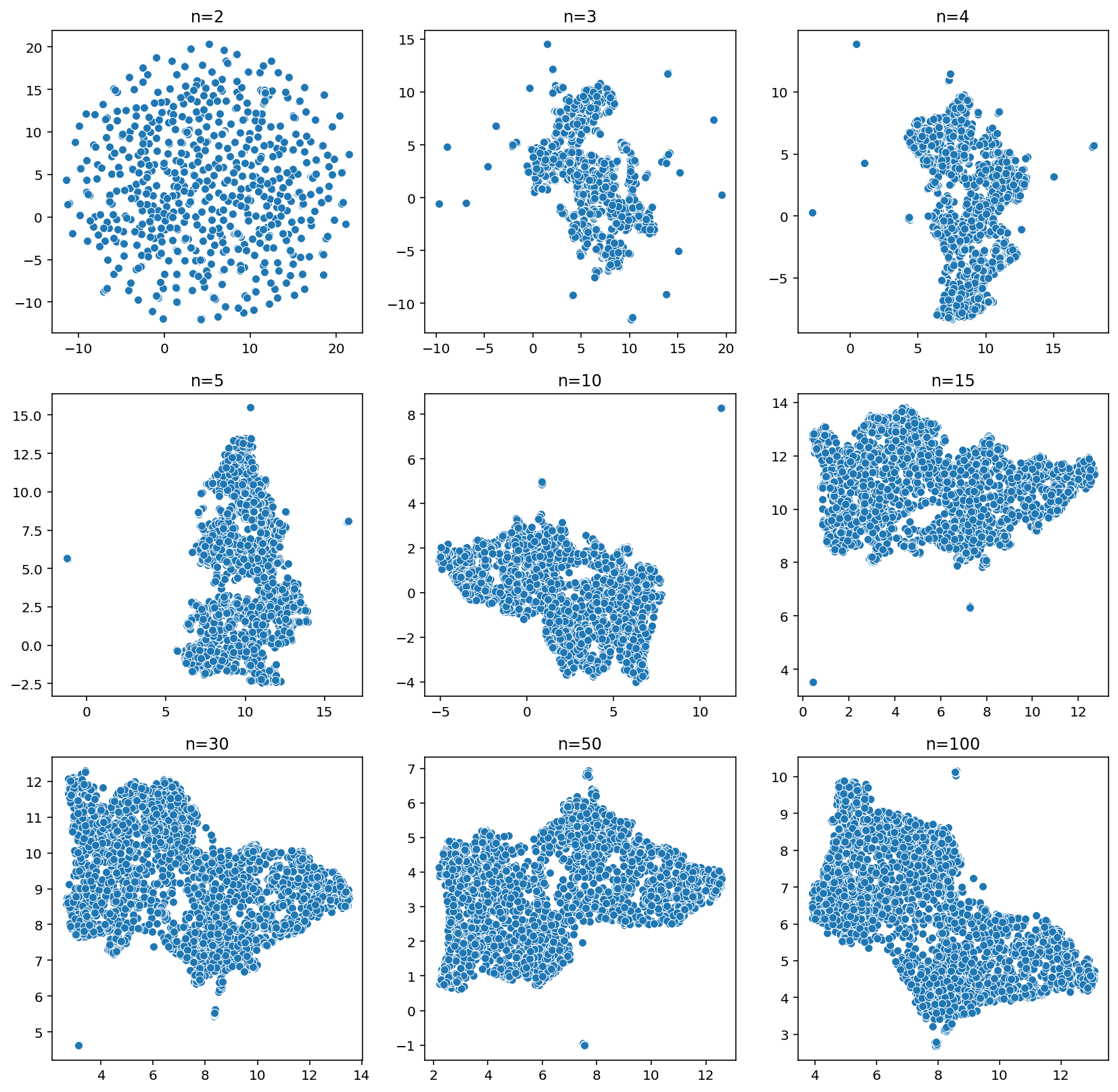
Hyperparameter search for n_neighbors

fig, ax = plt.subplots(3, 3, figsize=(14, 14))
nns = [2, 3, 4, 5, 10, 15, 30, 50, 100]
i, j = 0, 0
for n_neighbors in tqdm(nns):
    fit = umap.UMAP(n_neighbors=n_neighbors)
    u = fit.fit_transform(samples)
    sns.scatterplot(x=u[:,0], y=u[:,1], ax=ax[j, i])
    ax[j, i].set_title(f'n={n_neighbors}')
    if i < 2: i += 1
    else: i = 0; j += 1

OMP: Info #276: omp_set_nested routine deprecated, please use omp_set_max_active_levels instead.

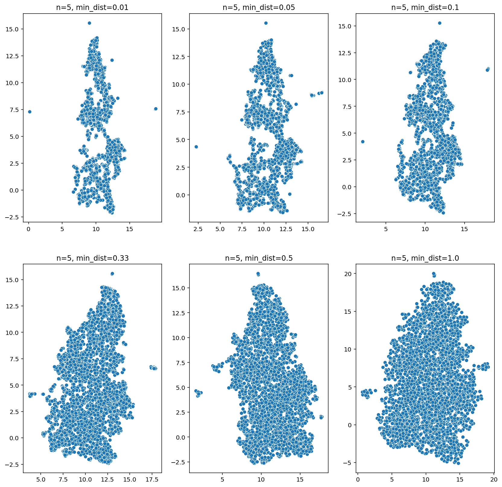
Hyperparameter search for min_dist

n_neighbors = 5

fig, ax = plt.subplots(2, 3, figsize=(14, 14))
min_dists = [0.01, 0.05, 0.10, 0.33, 0.5, 1.0]

i, j = 0, 0
for min_dist in tqdm(min_dists):
    fit = umap.UMAP(n_neighbors=n_neighbors, min_dist=min_dist)
    u = fit.fit_transform(samples)
    sns.scatterplot(x=u[:,0], y=u[:,1], ax=ax[j, i])
    ax[j, i].set_title(f'n={n_neighbors}, min_dist={min_dist}')
    if i < 2: i += 1
    else: i = 0; j += 1

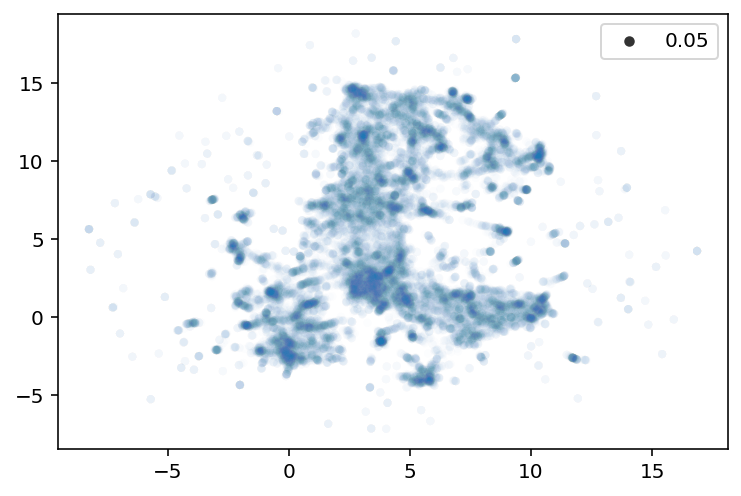
Fit UMAP

min_dist = 0.1
n_neighbors = 5

umap_fitter = umap.UMAP(n_neighbors=n_neighbors, min_dist=min_dist)
u = umap_fitter.fit_transform(embeddings)
sns.scatterplot(x=u[:,0], y=u[:,1], alpha=0.01, size=0.05)

<AxesSubplot:>

HDBSCAN

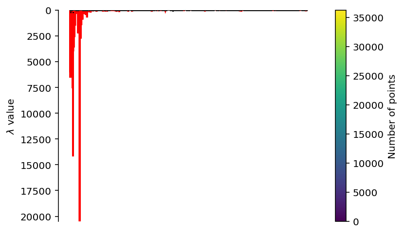
Clustering with defaults

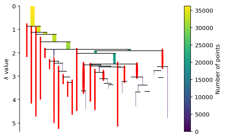
clusterer = hdbscan.HDBSCAN()
clusterer.fit(u)
clusterer.condensed_tree_.plot(select_clusters=True)

<AxesSubplot:ylabel='$\\lambda$ value'>

Clustering with optimized parameters

clusterer = hdbscan.HDBSCAN(
    min_cluster_size=200,
    min_samples=100,
    gen_min_span_tree=True,
    prediction_data=True
)
clusterer.fit(u)
clusterer.condensed_tree_.plot(select_clusters=True)

<AxesSubplot:ylabel='$\\lambda$ value'>

Custom BERTopic Model

BERTopic with customized models

import nltk
from nltk.corpus import stopwords
from sklearn.feature_extraction.text import CountVectorizer

nltk.download('stopwords')

stopwords = list(stopwords.words('english')) + ["covid", "covid 19", "19", "sars", "cov", "sars cov", "patients", "epidemic", "pandemic", "health", "sec", "sec sec"]
vectorizer_model = CountVectorizer(ngram_range=(1, 2), stop_words=stopwords)

if COMPUTE_TOPICS:
    topic_model = BERTopic(
        umap_model=umap_fitter,
        hdbscan_model=clusterer,
        embedding_model=embedding_model,
        vectorizer_model=vectorizer_model,
        calculate_probabilities=True,
        top_n_words=5,
        language='english',
        verbose=True
    )
    topics, probs = topic_model.fit_transform(sentences)
    topic_model.save(OUTPUT_FILE_TOPICS_BERTOPIC, save_embedding_model=False)
else:
  topic_model = BERTopic.load(OUTPUT_FILE_TOPICS_BERTOPIC)

Visualize topics

topic_model.visualize_barchart(top_n_topics=50)