MeWiKo-Co Dataset - Analysis of fine grained intent classification

Imports and Login

import pandas as pd

Load input data

df_refs = pd.read_csv(INPUT_FILE_REFS)\
            .dropna(subset=["contexts"])\
            .drop_duplicates(subset=["paperId", "contexts"])\
            .reset_index(drop=True)


df_multicite = pd.read_csv(INPUT_FILE_MULTICITE)\
                 .rename(columns={"label":"multicite_label", "score":"multicite_score"})
df = pd.concat([df_refs, df_multicite], axis=1)

Distribution of isInfluential

df.isInfluential.value_counts()

False    134195
True      73821
Name: isInfluential, dtype: int64

Distribution of intention classes

df.multicite_label.value_counts()
df.multicite_label.value_counts().plot(kind="bar")

<AxesSubplot:>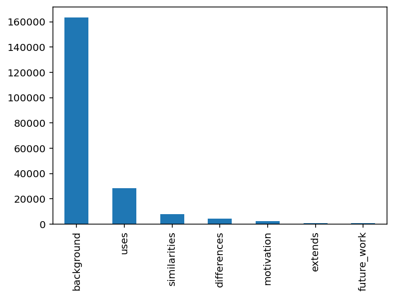

Intention classes by paper

df.pivot_table(index=pd.Grouper(key="doi"), columns=["multicite_label"], values=["multicite_score"], aggfunc="count")

	multicite_score
multicite_label	background	differences	extends	future_work	motivation	similarities	uses
doi
10.1101/2020.08.02.20129767	38.0	3.0	NaN	NaN	NaN	6.0	1.0
10.1101/2020.08.05.20169060	89.0	NaN	NaN	NaN	2.0	6.0	4.0
10.1101/2020.08.06.20168294	12.0	1.0	NaN	NaN	1.0	1.0	3.0
10.1101/2020.08.06.20169573	33.0	NaN	NaN	NaN	NaN	NaN	NaN
10.1101/2020.08.06.20169581	87.0	NaN	NaN	NaN	3.0	NaN	12.0
...	...	...	...	...	...	...	...
10.5194/se-2020-155	116.0	NaN	3.0	NaN	1.0	3.0	7.0
10.5194/se-2020-194	14.0	NaN	NaN	NaN	NaN	1.0	2.0
10.5194/se-2020-200	62.0	NaN	NaN	2.0	NaN	12.0	9.0
10.5194/se-2020-203	81.0	2.0	NaN	NaN	2.0	6.0	12.0
10.5194/tc-2020-330	16.0	1.0	NaN	1.0	NaN	3.0	6.0

5247 rows × 7 columns

Statistics of intention class occurences in papers

df.pivot_table(index=pd.Grouper(key="doi"), columns=["multicite_label"], values=["multicite_score"], aggfunc="count").describe()

	multicite_score
multicite_label	background	differences	extends	future_work	motivation	similarities	uses
count	5106.000000	1539.000000	415.000000	396.000000	1078.000000	2152.000000	3706.000000
mean	32.009597	2.957115	2.079518	1.631313	2.144712	3.623141	7.664868
std	40.483978	4.832646	2.119826	1.107136	1.796888	4.013191	10.844226
min	1.000000	1.000000	1.000000	1.000000	1.000000	1.000000	1.000000
25%	9.000000	1.000000	1.000000	1.000000	1.000000	1.000000	2.000000
50%	21.000000	2.000000	1.000000	1.000000	1.000000	2.000000	4.000000
75%	40.000000	3.000000	2.000000	2.000000	3.000000	4.000000	9.000000
max	885.000000	156.000000	31.000000	7.000000	15.000000	62.000000	218.000000

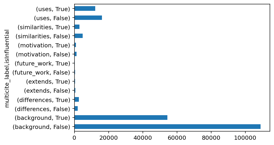
Distribution of intention class and isInfluential

df.groupby(by=["multicite_label", "isInfluential"])["multicite_label"].count().plot(kind="barh")

<AxesSubplot:ylabel='multicite_label,isInfluential'>

Intro